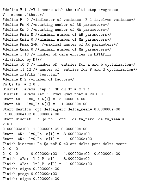
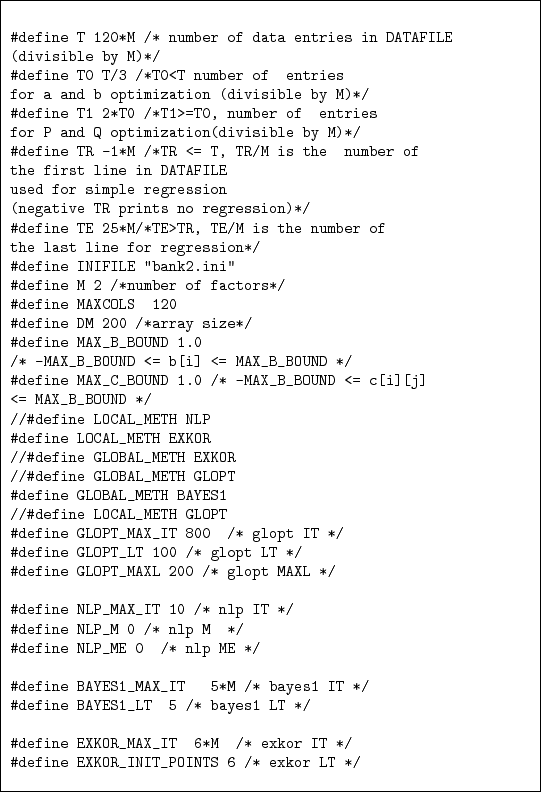
Figures 1.21 and 1.22 show the part of the file 'fitimeb.h' defining the control parameters and data files.
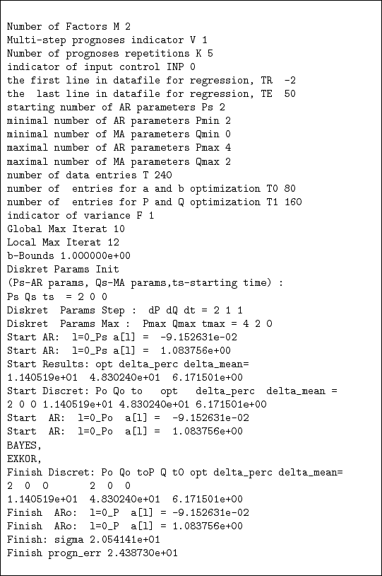
The control parameters and the optimization results (in the case INP 0) are shown in Figure 1.23. The comments in Figures 1.21 and 1.21 are short thus additional explanations are added.#define RAND() drand48(),defines the random number generator
#define S 0 /* number of rows of matrix c */
#define S 0 /* number of rows of matrix c */
defines the bilinear component (see expression 1.35)
#define K 5 /*number of "multi-step" repetitions*/,K 5 means that the multi-step predictions is repeated 5 times (see section 1.9 and Figure 1.24)
#define W 0 /*W 0 means the one-step structural optimization,
W 1 defines the multi-step one*/,
one-step structural optimization minimizes the average error of the "next day" predictions (see section 1.10.3), multi-step one minimizes the average error of predictions for longer periods of time
#define V 1 /*V 1 means with the multi-step prognoses,
V 0 means without*/
the zero value of the indicator V switches off the multi-step prediction (see section 1.9) and switches on the next day prediction (see section 1.3.3 and Figure 1.24)
#define F 1 /*indicator of variance, F 1 involves variance*/,the unit value of the indicator F means that the variance of the errors
#define EPS 0/*indicator of residual printing*/,not used in this version
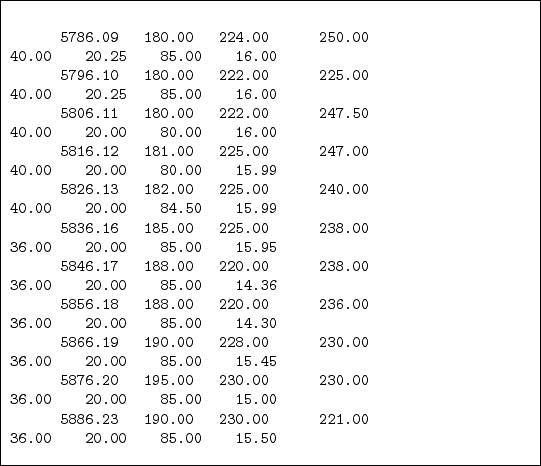
#define INP 0 /*indicator of input display*/,if INP 1 then the input values of the predicted factor are printed with their numbers (see Figure 1.25)
#define SA 0 /*indicator of simulated annealing */if SA 1 then optimization of the parameters p and q are performed using the simulated annealing method, otherwise the exhaustive search is used
#define PL 0/*plotting dimension*/,if PL 1 then the values of objective function depending on the parameter b[PLOT1] will be written in the file 'plot.out', if PL 2 then the values of objective function depending on two parameters b[PLOT1] and b[PLOT2] will be written in the file 'plot.out' (see Figure 1.26) and plotted as Figures 1.18 using the "Gnuplot" system,, if PL 0 there will be no file 'plot.out'
#define PLOT1 0 /*first plotting coordinate is b[PLOT1}*/
#define PLOT2 1/*second plotting coordinate is b[PLOT2}*/,
defines which components of vector-parameter b are considered
#define A1 -1.5 /*lower bound of  b[PLOT1}*/
#define B1 1.5/*upper bound of  b[PLOT2}*/
#define A2 -1.5 /*lower bound of  b[PLOT2}*/
#define B2 1.5/*upper bound of  b[PLOT2}*/
#define DN 50 /*number of plotting steps*/
defines the range and the density of the plotting points
#define ST 10000. /*temperature of simulated annealing */
#define SI 100 /*number of simulated annealing iterations*/
defines the parameters of simulated annealing method (if SA is applied)
#define Ps M  /*starting number of AR parameters*/
#define Qs 0  /*starting number of MA parameters*/
#define Pmin M /*minimal number of AR parameters*/
#define Qmin 0  /*minimal number of MA parameters*/
#define Pmax 2*M  /*maximal number of AR parameters*/
#define Qmax 2  /*maximal number of MA parameters*/
defines the initial, the minimal and the maximal number of parameters p and q in the structural optimization
#define T 120*M /* number of data entries in DATAFILE
(divisible by M)*/,
defines the total number of entries in DATAFILE
#define T0 T/3 /*T0<T number of  entries
for a and b optimization (divisible by M)*/
#define T1 2*T0 /*T1>=T0, number of  entries
for P and Q optimization(divisible by M)*/,
divides the DATAFILE (see Figures 1.27 and 1.17) into three parts: the first part for a,b optimization, the second part for p,q optimization, and the third part for testing the results
 |
#define TR -1*M /*TR <= T, TR/M is the  number of
the first line in DATAFILE used for simple regression
(negative TR prints no regression)*/
#define TE 25*M/*TE>TR, TE/M is the number of
the last line for regression*/,
is used only in the case when the ARMA model of time series prediction is reduced to the linear regression model of diagnosis.
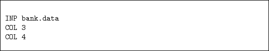
#define INIFILE "bank2.ini",defines the input control file INIFILE (see Figure 1.28)
#define M 2 /*number of factors*/,defines the number of factors, including the predicted and the external ones
#define LOCAL_METH EXKOR,means that the EXKOR method is used for local optimization
#define GLOBAL_METH BAYES1means that the BAYES1 method is used for global optimization
#define BAYES1_MAX_IT  	5*M	/* bayes1 IT */
#define BAYES1_LT	 5	/* bayes1 LT */
means that 5*M iterations and 5 initial iterations of the BAYES1 method are used
#define EXKOR_MAX_IT	 6*M 	/* exkor IT */
#define EXKOR_INIT_POINTS 6	/* exkor LT */
means that 6*M iterations and 6 initial iterations of the EXKOR method are used
![\begin{figure}\begin{codebox}{4.7in}
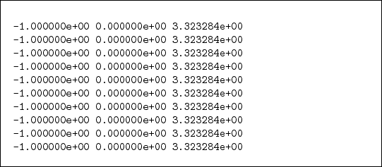
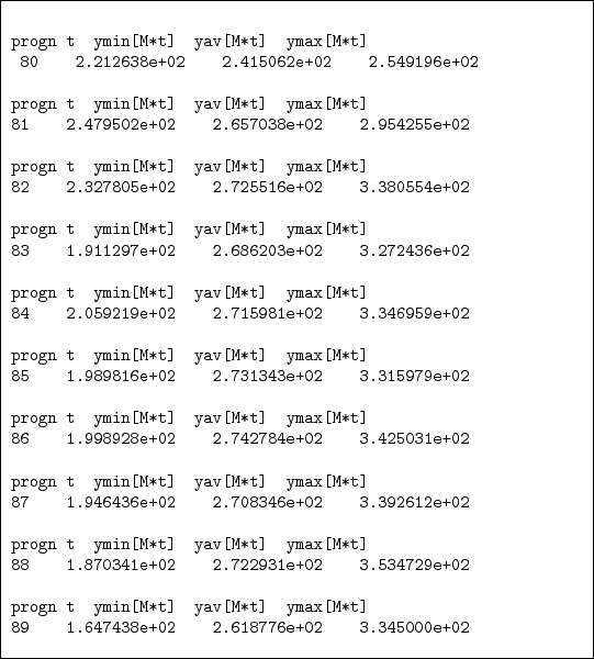
\begin{verbatim}progn t ymin[M*t] yav[M*t...
... 1.647438e+02 2.618776e+02 3.345000e+02\end{verbatim}
\end{codebox}
\end{figure}](img288.png)