


Next: Optimization Results
Up: Examples of Squared Residuals
Previous: Examples of Squared Residuals
Consider, as some illustrations
- exchange rates of $/
 , DM/$, yen/$, and franc/$
- closing rates of stocks of AT&T, Intel Corporation, and Hermis bank
![[*]](file:/usr/share/latex2html/icons/footnote.png)
- London stock exchange index
- daily call rates of a call center.
The figures show the data and corresponding optimization results. The optimization results demonstrate how least square deviations depend on parameters  of ARMA models. The optimization results are presented in two forms: as
surfaces and as contours.
of ARMA models. The optimization results are presented in two forms: as
surfaces and as contours.
Figures 1.5, 1.6, and 1.7 consider exchange rates of $/ and DM/$.
Figures 1.8, 1.9, and 1.10 regard exchange rates of yen/$ and franc/$.
Figures 1.11, 1.12, and 1.13 reflect closing rates of AT&T and Intel Co. stocks.
Figures 1.14 , 1.15, and 1.16 consider the London stock exchange index.
Figures 1.17, 1.18, and 1.18 shows stock rates of the Hermis bank and optimization results.
Figures 1.19 and 1.20 show the daily call rates of a call center and illustrate optimization results.
Figure 1.5:
Daily exchange rate of $/£(top figure) and DM/$ (bottom figure) starting from September 13, 1993
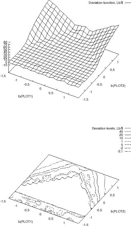 |
Figure 1.6:
Exchange rates of £/$:
surface  depending on parameters
  (top),
contours of depending on parameters (bottom)
(top),
contours of depending on parameters (bottom)
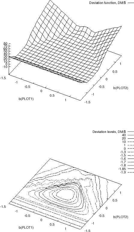 |
Figure 1.7:
Exchange rates of DM/$:
surface of depending on
parameters (top),
contours of depending on parameters (bottom)
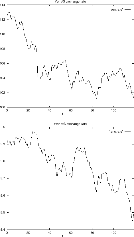 |
Figure 1.8:
Exchange rates:
yen/$ (top), franc/$ (bottom)
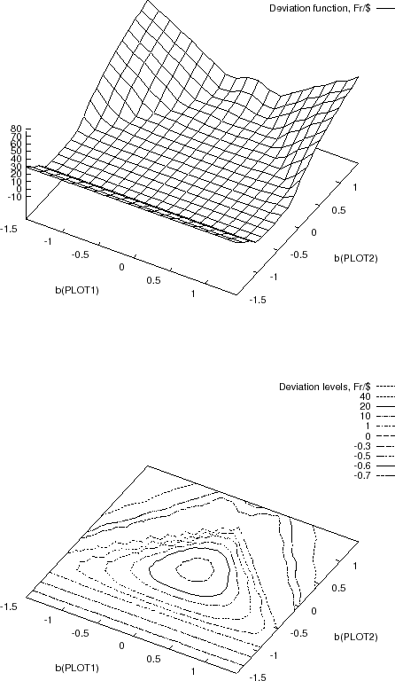 |
Figure 1.9:
Exchange rates of fr/$,
surface depending on parameters (top),
contours of depending on parameters (bottom)
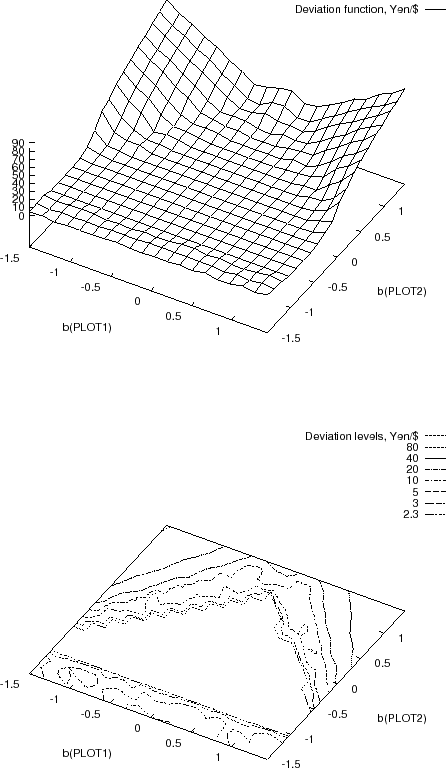 |
Figure 1.10:
Exchange rates of yen/$,
surface depending on parameters (top),
contours of depending on parameters (bottom)
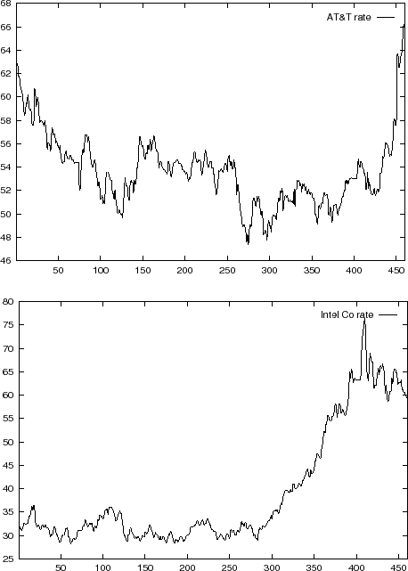 |
Figure 1.11:
AT&T (top) and Intel Co.(bottom) stocks closing rates starting from August 30, 1993
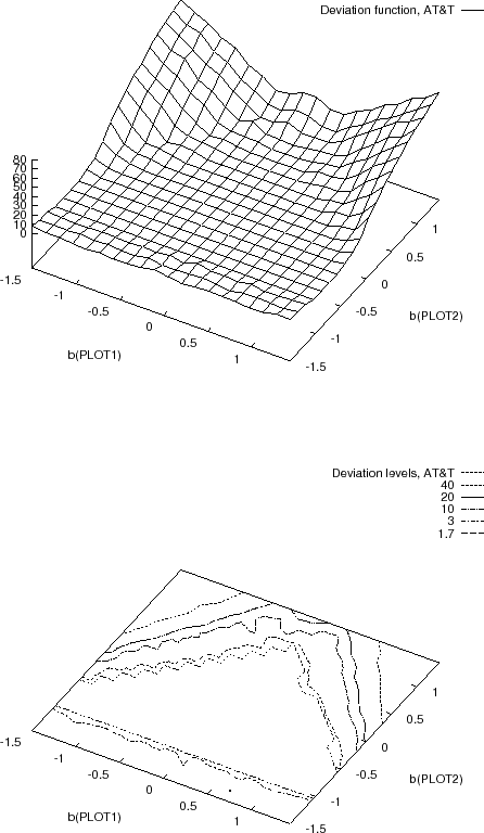 |
Figure 1.12:
Closing rates of AT&T stocks:
surface depending on parameters (top),
contours of depending on parameters (bottom)
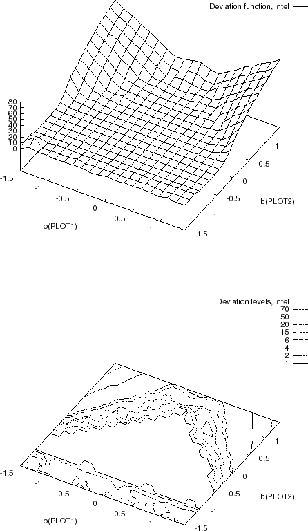 |
Figure 1.13:
Closing rates of Intel Co stocks:
surface of depending on parameters (top)
contours of depending on parameters (bottom)
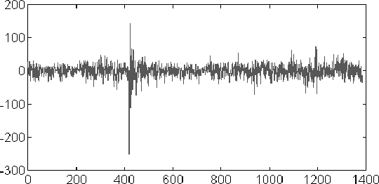 |
Figure 1.14:
London stock exchange index
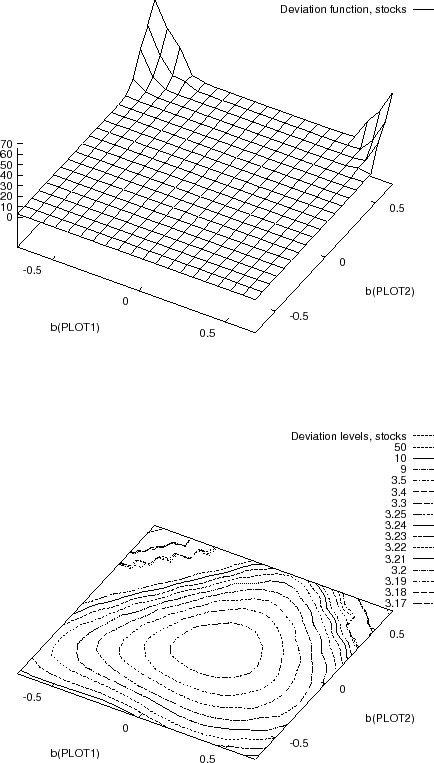 |
Figure 1.15:
London stock exchange index,
surface of depending on
parameters (top),
contours of depending on parameters (bottom)
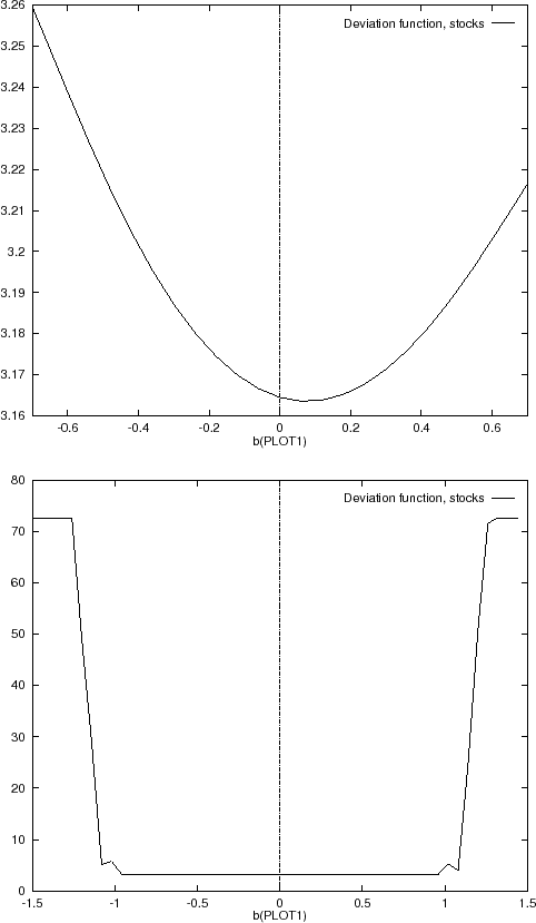 |
Figure 1.16:
London stock exchange index:
deviation depending on parameter  , uni-modal part (top),
multi-modal part (bottom)
, uni-modal part (top),
multi-modal part (bottom)
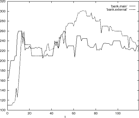 |
Figure 1.17:
Closing rates of stocks of
the Hermis bank (private) and the Lithuanian Savings bank (state)
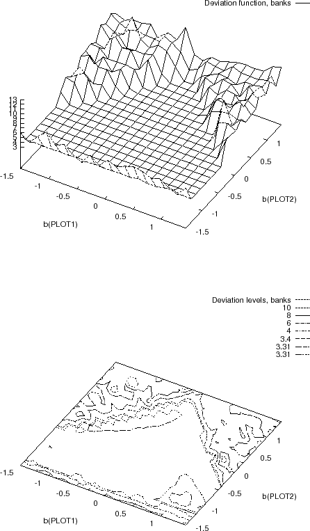 |
Figure 1.18:
Closing rates of Hermis bank stocks:
surface of depending on parameters (top)
contours of depending on parameters (bottom)
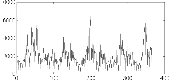 |
Figure 1.19:
Call rates.
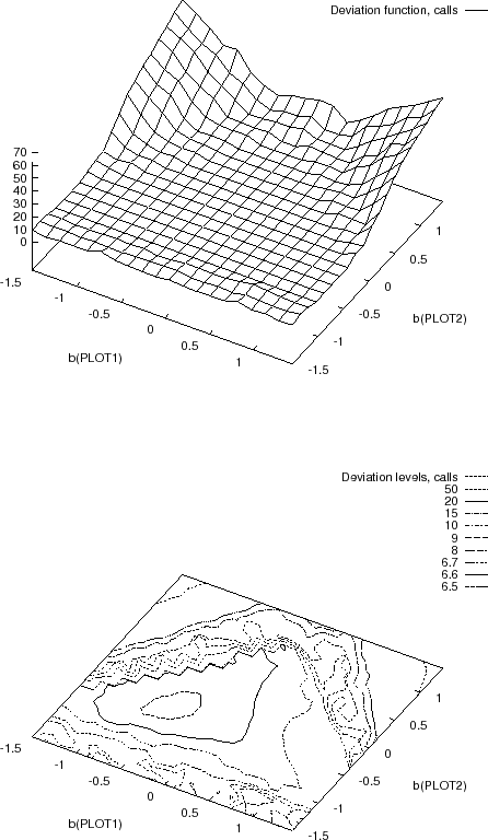 |
Figure 1.20:
Call rates: surface of depending on
parameters (top),
contours of depending on parameters (bottom).
 |
Estimating unknown ARMA parameters
we minimize a log-sum of squared residuals
defined by expression (1.45).
Parameters  are estimated by expression (1.13).
The figures indicate the multi-modality of log-sum (1.45) as a function of
parameters in most of the cases.
Areas in vicinity of the global minima often appear flat.
A reason is that differences between values of the deviation function in an areas around the global minimum are smaller as compared with these outside this area (see Figures 1.16).
are estimated by expression (1.13).
The figures indicate the multi-modality of log-sum (1.45) as a function of
parameters in most of the cases.
Areas in vicinity of the global minima often appear flat.
A reason is that differences between values of the deviation function in an areas around the global minimum are smaller as compared with these outside this area (see Figures 1.16).
Next: Optimization Results
Up: Examples of Squared Residuals
Previous: Examples of Squared Residuals
mockus
2008-06-21