In this section the insurance model of multiple objects ![]() is reduced to
that of a single object.
Some companies apply "zero-one" insurance policies:
is reduced to
that of a single object.
Some companies apply "zero-one" insurance policies: ![]() or
or ![]() .
In this case no equilibrium exist because only
two discrete strategies can be applied2.
If a number of customers is large,
for example a set of car owners, one approximates discrete set
by the continuous one assuming that
.
In this case no equilibrium exist because only
two discrete strategies can be applied2.
If a number of customers is large,
for example a set of car owners, one approximates discrete set
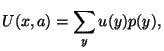
by the continuous one assuming that ![]() is a sum of
insurance policies of
is a sum of
insurance policies of
![]() customers that decided to
insure their property
customers that decided to
insure their property
![]() .
Here
.
Here ![]() is a number of customers that decided to insure
their objects including
is a number of customers that decided to insure
their objects including ![]() insured survivors.
Then
insured survivors.
Then ![]() is a number of not insured objects including
is a number of not insured objects including
![]() of not insured survivors.
of not insured survivors.
Assume as a first approximation that
Under these assumptions the expected cumulative utility
Suppose that total wealth of all customers
![]() .
.
From (26)
From the assumption that survival probabilities ![]() of all the objects3 are
equal and independent follows the binomial distribution.
If
of all the objects3 are
equal and independent follows the binomial distribution.
If ![]() , where
, where ![]() , is
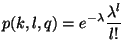
not very large and not very small then one approximates the binomial distribution by the Poisson
distribution . The probability that
, is
not very large and not very small then one approximates the binomial distribution by the Poisson
distribution . The probability that ![]() of
of ![]() objects survive and the rest
objects survive and the rest ![]() do not
do not
 |
(29) |
| (30) |
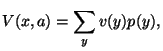
The expected utility ![]() of insurance company
is defined in a similar way.
of insurance company
is defined in a similar way.
Suppose that
![]() .
.
From (26)
From here and assumption (26)
the probability ![]() of profit
of profit
![]()
| (33) |
Here insurance policy ![]() is defined indirectly
by the number of customers
is defined indirectly
by the number of customers ![]() that insure their of objects
maximizing their expected cumulative utility
(15) that depends on the rate of insurance charge
that insure their of objects
maximizing their expected cumulative utility
(15) that depends on the rate of insurance charge ![]() .
This is a correct assumption if the cumulative utility function
.
This is a correct assumption if the cumulative utility function
![]() represents individual utilities
represents individual utilities ![]() well enough.
Therefore definition of
well enough.
Therefore definition of ![]() is important part of model
that represents multiple customers as a single one.
is important part of model
that represents multiple customers as a single one.
The equilibrium between interests of the company and the customer
is achieved when both insurance policy ![]() and
insurance charge
and
insurance charge ![]() satisfies Nash conditions.
One obtains the Nash equilibrium using the same expressions as in
the previous section.
satisfies Nash conditions.
One obtains the Nash equilibrium using the same expressions as in
the previous section.