Discussions

Table 1.2 shows some results obtained using the ARFIMA model [14]. Parameters $b$ and $d$ were estimated using daily exchange rates of $/£, and DM/$, and closing rates of AT&T and Intel Co stocks.

Table 1.2: Estimated parameters $b$ and $d$ of ARFIMA models.

$Data$	$b_0$	$b_1$	$d$	$\min \log f(x)$
$/$\pounds$	-1.195	-0.169	0.0005	1.51675
DM/$	-1.019	0.0120	0.0007	1.60065
AT&T	-1.017	0.0118	0.00005	9.83208
Intel Co	0.9975	0.0055	0.012	7.35681

It is clear from Table 1.2 that $d$'s for all the time series are very close to zero (see also Figures 1.3 and 1.4).

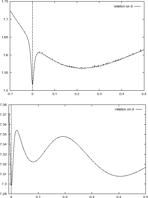
Figure 1.3: Log-sum (1.45) as a function of the parameter $d \in [-0.1,0.5]$ regarding the $/$\pounds$ exchange rate
Figure 1.4: Log-sum (1.45) as a function of the parameter $d \in [-0.01,0.5]$ regarding the Intel Co stocks closing rate

Hence, following the traditional approaches to testing for long memory processes (see, for example,[1,20,2]) we may conclude that the underlying stochastic processes generating exchange rates of $/£and DM/$ , and closing rates of AT&T and Intel Co stocks, do not exhibit persistence and are stationary. That contradicts the visual impression of the corresponding data (see Figures 1.5 and 1.11). This apparent contradiction may be resolved by dropping the assumption that the parameters $a,b,d$ of the ARFIMA model remain constant. This assumption is common for most of the traditional methods. An alternative is structural stabilization models described in chapter 1.10.