The traditional time series models assume that their parameters do not change. Examples are parameters ![]() of the ARMA model, parameters
of the ARMA model, parameters ![]() of the ARFIMA model, parameters
of the ARFIMA model, parameters ![]() of the BL model, and parameters
of the BL model, and parameters
![]() of the ANN model.
of the ANN model.
The variability of parameters of models describing the financial data such as stock rates and the currency exchange rates can be partially explained by the changes of economical conditions. However this variability is there even in the stable economical conditions. The reason is the "Feed-Back" processes. It is well known that the predictions may influence the supply and demand and consequently the future data.. In such cases the statistical best fit models should be complemented or replaced by the game-theoretical equilibrium models. However there is the possibility that the equilibrium model would be namely the Wiener process. That means that the market rates in economics are governed by the similar model as the Brownian motion in physics and are as unpredictable as the movement of individual molecules in gases. Table 1.1 shows that the simplest Wiener process, called as the Random Walk (RW), predicts the financial data at least as well as Arma models.
The objective of traditional time series models is to define such parameters that minimize a deviation from the available data.
One may call them as the best fit models.
The goodness of fit is described by continuous parameters ![]() called as state variables. For example, in the ARMA model (see expression (1.1)) the state variables
called as state variables. For example, in the ARMA model (see expression (1.1)) the state variables
![]() .
.
If the parameters remain constant in the future, then models that fit best to the past data will predict the future data as well. Otherwise, the best fit to the past data can be irrelevant or even harmful for predictions.
Models are needed which are not sensitive to the changes of system parameters. Such models may predict the uncertain future better by eliminating the nuisance parts from the structure of the model.
Trying to solve this problem we introduce a notion of the model structure. The model structure is determined by the Boolean parameters
![]() called as structural variables. A structural variable is equal to unit if the corresponding component of time series model is included . Otherwise, the structural variable is equal to zero. For example, in the ARMA model
called as structural variables. A structural variable is equal to unit if the corresponding component of time series model is included . Otherwise, the structural variable is equal to zero. For example, in the ARMA model
![]() . Here
. Here
![]() , if the parameter
, if the parameter ![]() is included into the ARMA model and
is included into the ARMA model and ![]() , otherwise
, otherwise![]() .
We search for such structure
.
We search for such structure ![]() of the model that minimizes the prediction errors in the changing environment.
of the model that minimizes the prediction errors in the changing environment.
To achieve this we divide available data
![]() into two parts
into two parts
![]() and
and
![]() .
.
The first part ![]() is for estimation of continuous parameters
is for estimation of continuous parameters ![]() which depends on Boolean structural parameters
which depends on Boolean structural parameters ![]() . The estimation is performed for a set of all feasible
. The estimation is performed for a set of all feasible ![]() by minimizing the least square deviation.
by minimizing the least square deviation.
The second part ![]() is used to select such
is used to select such ![]() that
minimize the least square deviation. This means that the second part
that
minimize the least square deviation. This means that the second part ![]() is for estimation of Boolean structural parameters.
is for estimation of Boolean structural parameters.
Denote by ![]() the predicted value of a model
the predicted value of a model ![]() with fixed parameters
with fixed parameters ![]() using the data
using the data
![]() . The difference between the prediction and the actual data
. The difference between the prediction and the actual data ![]() is denoted by
is denoted by
![]() . Denote by
. Denote by ![]() the fitting parameters
the fitting parameters ![]() which minimize the sum of squared deviations
which minimize the sum of squared deviations
![]() using the first data set
using the first data set ![]() at fixed structure parameters
at fixed structure parameters ![]() .
.
We consider two data sets ![]() and
and ![]() just for simplicity.
One may partition the data
just for simplicity.
One may partition the data ![]() into many data subsets
into many data subsets
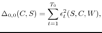
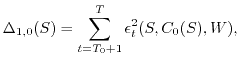
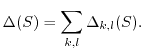
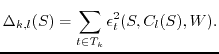
![]() . In this case we minimize the sum
. In this case we minimize the sum
 |
(53) |
 |
(54) |
The usefulness of the structural stabilization follows from the observation that any optimal
estimate of time series parameters using a part ![]() of the data
of the data
![]() is optimal for another part
is optimal for another part ![]() only if all the parameters remain the same. Otherwise one may obtain a better estimate eliminating the changing parameters from the model. For example in the case of changing parameters
only if all the parameters remain the same. Otherwise one may obtain a better estimate eliminating the changing parameters from the model. For example in the case of changing parameters
![]() of the ARMA model the best prediction may be obtained by elimination of all the parameters except
of the ARMA model the best prediction may be obtained by elimination of all the parameters except ![]() (see Table 1.1).
(see Table 1.1).